
Primary Exploration of the Basin Effect on Significant Duration
-
摘要: 利用关东盆地及其周边KiK-net台网井上台站记录的2004—2017年15次中强地震(矩震级为5.1~6.9级)构建三分量记录显著持时Ds5-95数据库。针对该数据库,基于残差分析方法和3种水平向地震动持时参数预测方程,计算并给出事件间残差和事件内残差及其随不同类别参数的变化。在此基础上,初步探讨了水平向地震动持时预测方程应用于预测竖向地震动持时的可行性及盆地对三分量地震动持时的影响。研究结果表明,对于震源距和场地VS30相当的情况,盆地内台站持时普遍大于盆地外台站持时,盆地内、外台站竖向地震动持时均大于水平向地震动持时;3种预测方程均可实现对盆地外台站水平向地震动Ds5-95的合理估计,但在一定程度上低估了盆地内台站的水平向地震动Ds5-95;3种预测方程均无法直接应用于竖向地震动持时预测。Abstract: Based on the three-component records of MW 5.1~MW6.9 earthquake events recorded by KiK-net of Japan Strong Motion Observatory Network from 2004 to 2017, this paper constructs the Ds5-95 duration database of 15 strong crustal earthquakes in the Kanto basin. Further, the inter-event residuals and intra-event residuals of the duration database are calculated based on the residual analysis method and three kinds of duration prediction equations, and their changes with different parameters are also discussed. The prediction level of vertical earthquake ground motion duration based on duration prediction equation for horizontal ground motion and the influence of basin on three component earthquake records duration are analyzed. The results show that the duration of earthquake ground motion for inside-basin stations is greater than that of outside-basin stations, and the duration of vertical earthquake ground motion is greater than that of horizontal ground motion, thus, the influence of the basin effect on the duration can not be ignored; Three kinds of duration prediction equations can realize the reasonable estimation of horizontal earthquake ground motion Ds5-95 duration for outside-basin stations, but to a certain extent, horizontal earthquake ground motion Ds5-95 duration is underestimated for inside-basin stations; Three kinds of duration prediction equations can not be directly applied to the estimation of vertical earthquake ground motion duration.
-

图 1 震中-台站方位的分布
Figure 1. Orientation distribution of earthquake epicenters and stations
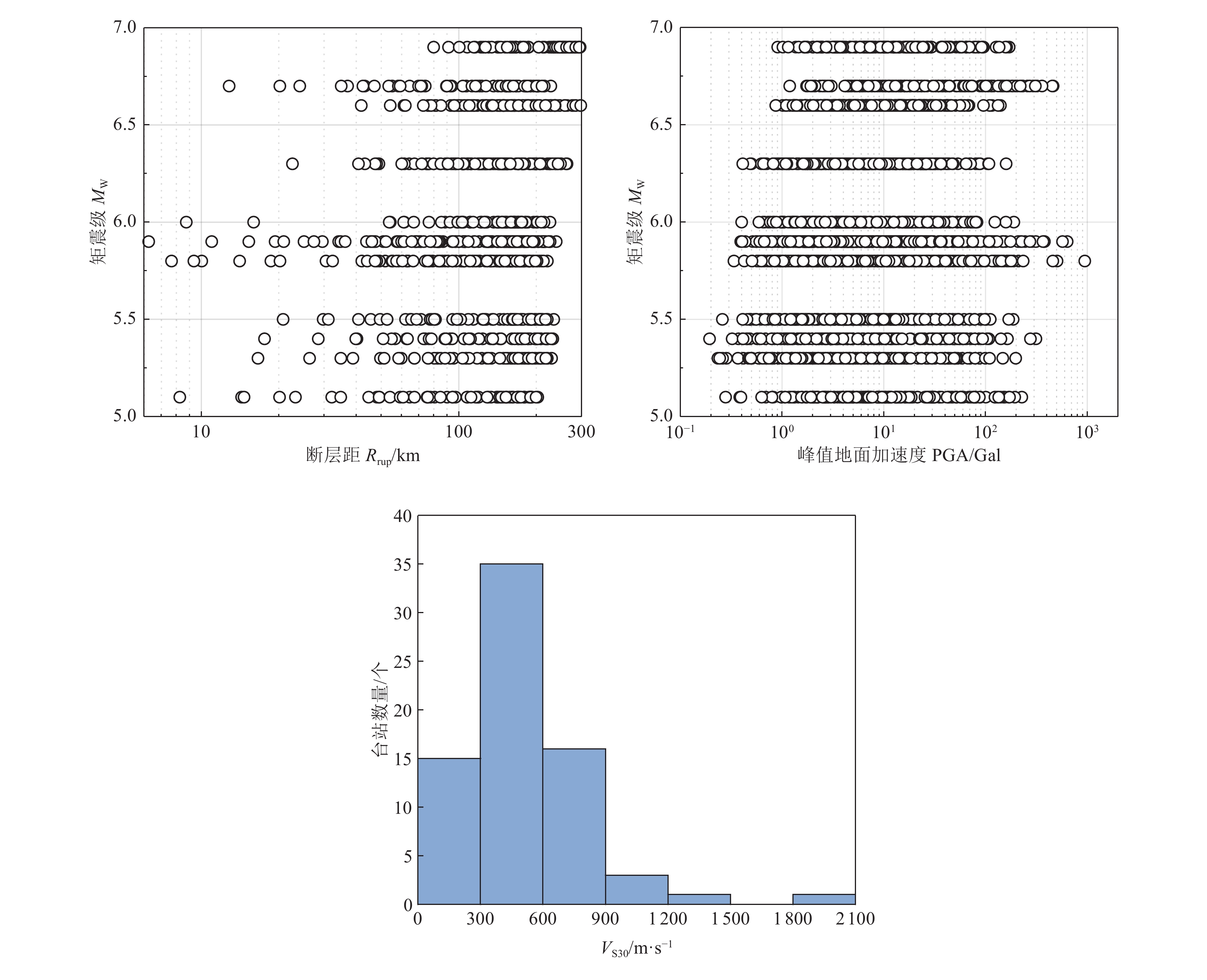
图 2 构建持时数据库中各参数的分布情况
Figure 2. Distribution of parameters in constructed duration database
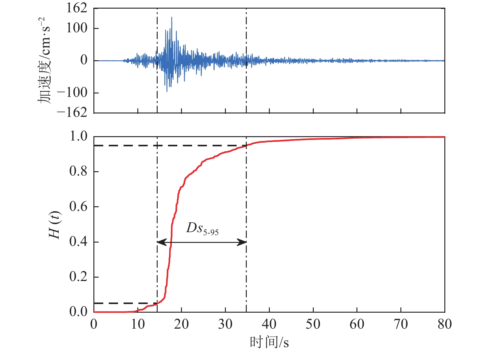
图 3 Ds5-95计算示意及Husid函数
Figure 3. Significant duration Ds5-95 using the Husid plot for acceleration time history

图 4 三分量地震动记录显著持时Ds5-95随断层距Rrup的分布
Figure 4. Distribution of significant duration Ds5-95 for three-component ground motion records versus rupture distance Rrup

图 5 不同持时预测方程显著持时Ds5-95的事件间残差随矩震级的变化
Figure 5. The inter-event residual and of significant duration Ds5-95 versus moment magnitude MW in different duration ground motion prediction equations

图 6 不同持时预测方程显著持时Ds5-95的事件内残差及分组均值标准差随断层距的变化
Figure 6. The intra-event residual and their binned means and ±1 standard deviations of significant duration Ds5-95 versus rupture distance Rrup in different duration ground motion prediction equations
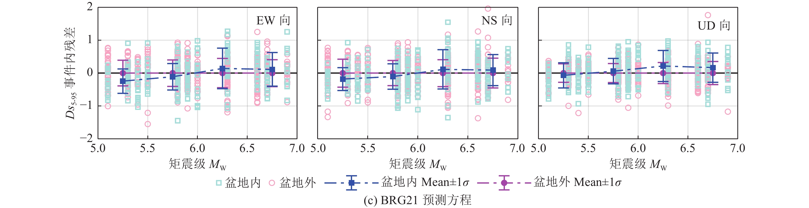
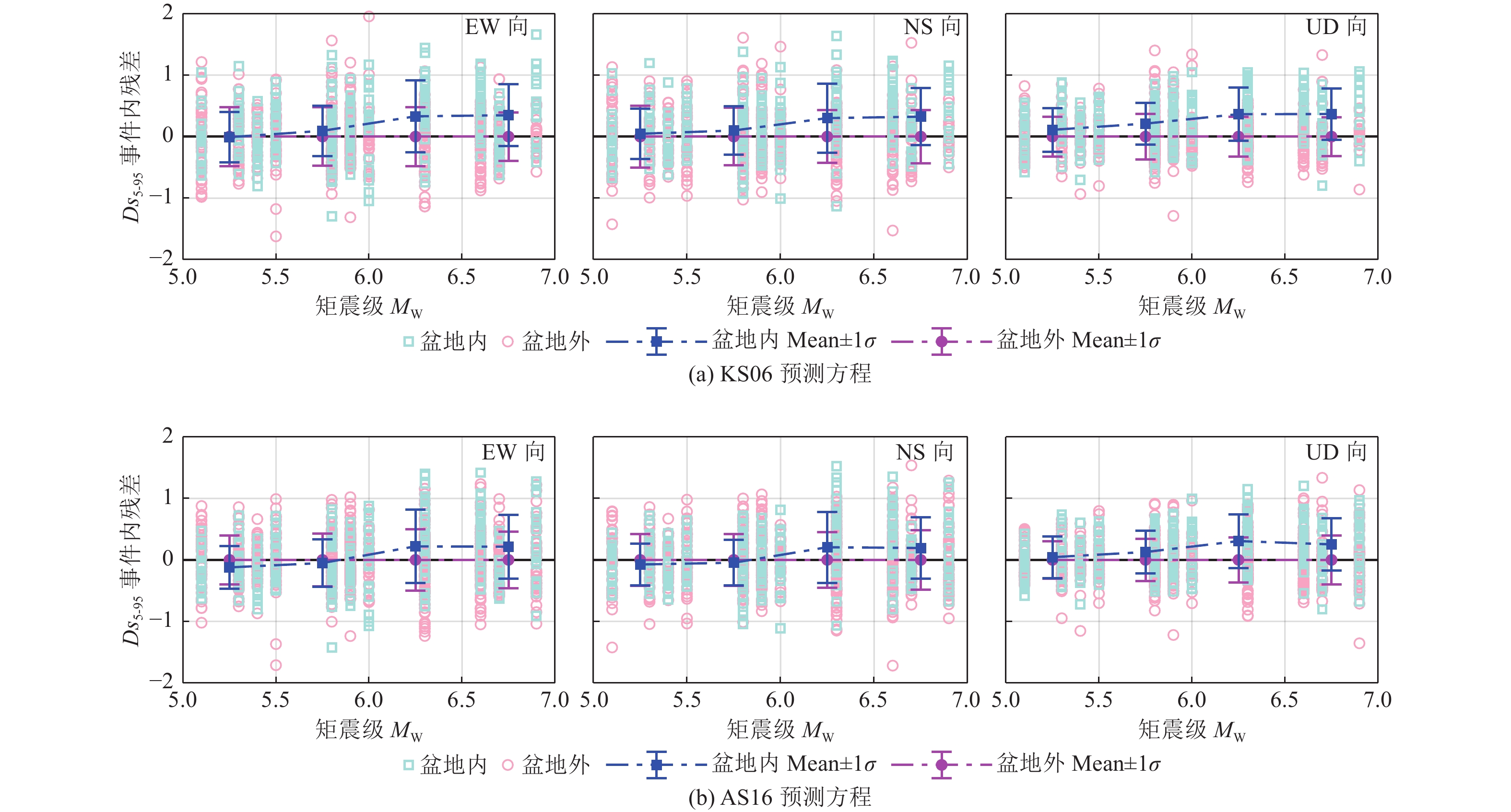
7 不同持时预测方程显著持时Ds5-95的事件内残差及分组均值标准差随矩震级的变化。
7. The intra-event residual and their binned means and ±1 standard deviations of significant duration Ds5-95 versus moment magnitude Mw in different duration ground motion prediction equations
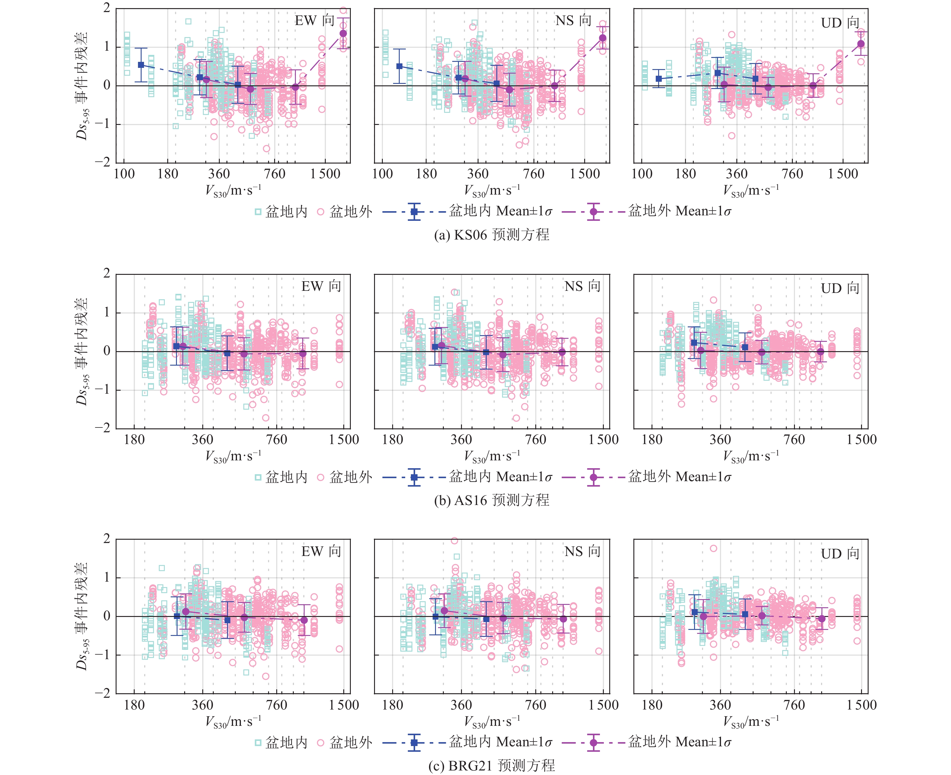
图 8 不同持时预测方程显著持时Ds5-95的事件内残差及分组均值标准差随VS30的变化
Figure 8. The intra-event residual and their binned means and ±1 standard deviations of significant duration Ds5-95 versus VS30 in different duration ground motion prediction equations
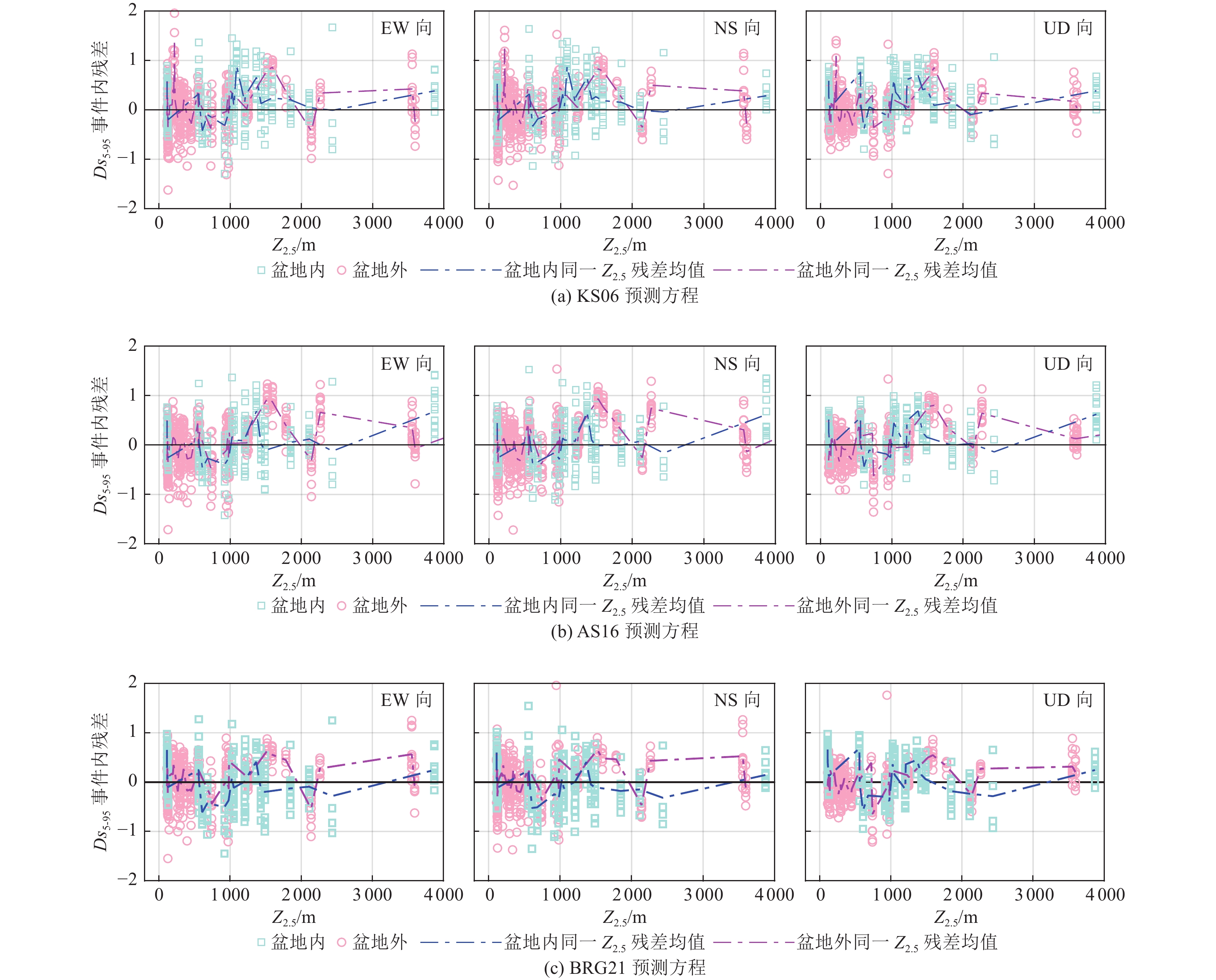
图 9 不同持时预测方程显著持时Ds5-95的事件内残差及同一Z2.5值对应的残差均值随Z2.5的变化
Figure 9. The intra-event residual and mean residual of the same Z2.5 value of significant duration Ds5-95 versus Z2.5 in different duration ground motion prediction equations
表 1 地震基本信息
Table 1. Information of selected crustal earthquakes
发震时间 矩震级MW 震中纬度/ ° 震中经度/ ° 断层距范围/ km 事件台站数量/ 个 事件记录总数/ 条 2004年10月23日17时56分 6.6 37.289 5 138.870 3 41.8~258.4 62 186 2004年10月23日18时34分 6.3 37.303 3 138.933 2 48.0~263.3 61 183 2007年07月16日10时13分 6.6 37.556 8 138.609 5 72.8~297.7 63 189 2011年03月12日03时59分 6.3 36.986 0 138.597 8 22.6~248.4 62 186 2011年03月16日12时52分 5.8 35.837 0 140.906 5 10.0~220.8 60 180 2011年03月19日18时56分 5.8 36.783 7 140.571 5 7.7~201.4 64 192 2011年04月11日17时16分 6.7 36.945 7 140.672 7 12.8~227.7 65 195 2011年04月11日20时42分 5.5 36.966 0 140.635 0 20.8~233.7 64 192 2011年04月12日14时07分 5.9 37.052 5 140.643 5 25.1~239.0 65 195 2011年04月13日10时08分 5.3 36.915 0 140.709 7 16.6~229.3 64 192 2012年03月14日21时05分 6.0 35.747 7 140.932 0 8.7~226.1 61 183 2013年09月20日02时25分 5.4 37.051 3 140.695 3 17.6~231.8 59 177 2016年11月22日05时59分 6.9 37.354 7 141.604 2 79.9~296.0 64 192 2016年12月28日21时38分 5.9 36.720 2 140.574 2 6.2~203.4 64 192 2017年08月02日02时02分 5.1 36.803 5 140.535 2 8.3~202.6 61 183  下载: 导出CSV
表 2 台站基本信息
Table 2. Information of selected stations inside and outside Kanto basin
台站编码 位于盆地内外情况 纬度/ ° 经度/ ° 台站编码 位于盆地内外情况 纬度/ ° 经度/ ° CHBH06 盆地内 35.721 5 140.504 6 GNMH12 盆地外 36.144 0 138.912 9 CHBH10 盆地内 35.545 8 140.241 7 GNMH13 盆地外 36.862 0 139.062 7 CHBH13 盆地内 35.830 7 140.298 0 GNMH14 盆地外 36.493 1 139.321 9 CHBH14 盆地内 35.734 2 140.823 0 IBRH06 盆地外 36.880 9 140.654 5 GNMH05 盆地内 36.314 3 139.184 7 IBRH11 盆地外 36.370 1 140.140 1 GNMH11 盆地内 36.286 2 138.921 0 IBRH12 盆地外 36.836 9 140.318 1 IBRH07 盆地内 35.952 1 140.330 1 IBRH13 盆地外 36.795 5 140.575 0 IBRH10 盆地内 36.111 2 139.988 9 IBRH14 盆地外 36.692 2 140.548 4 IBRH17 盆地内 36.086 4 140.314 0 IBRH15 盆地外 36.556 6 140.301 3 IBRH18 盆地内 36.363 1 140.619 8 IBRH16 盆地外 36.640 5 140.397 6 IBRH19 盆地内 36.213 7 140.089 3 KNGH11 盆地外 35.404 0 139.353 9 IBRH20 盆地内 35.828 4 140.732 3 KNGH18 盆地外 35.643 7 139.128 3 KNGH10 盆地内 35.499 1 139.519 5 KNGH19 盆地外 35.417 3 139.043 6 SITH03 盆地内 35.899 0 139.384 3 KNGH20 盆地外 35.366 3 139.126 0 SITH04 盆地内 35.802 8 139.535 3 KNGH21 盆地外 35.462 8 139.214 6 SITH06 盆地内 36.113 1 139.289 4 KNGH22 盆地外 35.358 3 139.091 0 TCGH06 盆地内 36.445 8 139.950 9 NGNH17 盆地外 36.142 5 138.550 4 TCGH10 盆地内 36.857 8 140.022 5 NGNH19 盆地外 35.973 5 138.584 5 TCGH12 盆地内 36.695 9 139.984 2 NIGH19 盆地外 36.811 4 138.784 9 TCGH13 盆地内 36.734 2 140.178 1 SITH05 盆地外 36.150 9 139.050 4 TCGH15 盆地内 36.559 5 139.863 7 SITH07 盆地外 35.911 8 139.148 5 TCGH16 盆地内 36.548 0 140.075 1 SITH08 盆地外 36.027 4 138.969 1 CHBH11 盆地外 35.286 7 140.152 9 SITH09 盆地外 36.071 5 139.099 3 CHBH12 盆地外 35.344 5 139.855 4 SITH10 盆地外 35.996 4 139.219 1 CHBH15 盆地外 34.959 1 139.788 5 SITH11 盆地外 35.863 7 139.272 6 CHBH16 盆地外 35.138 4 139.964 9 TCGH07 盆地外 36.881 7 139.453 4 CHBH17 盆地外 35.171 4 140.339 8 TCGH08 盆地外 36.882 8 139.645 9 CHBH20 盆地外 35.088 2 140.099 7 TCGH09 盆地外 36.862 5 139.836 4 FKSH05 盆地外 37.254 4 139.872 5 TCGH11 盆地外 36.708 4 139.769 4 FKSH06 盆地外 37.172 3 139.519 9 TCGH14 盆地外 36.550 9 139.615 4 FKSH10 盆地外 37.161 6 140.093 0 TCGH17 盆地外 36.985 3 139.692 2 FKSH13 盆地外 36.995 1 140.585 3 TKYH12 盆地外 35.670 1 139.265 0 GNMH07 盆地外 36.699 8 139.210 4 TKYH13 盆地外 35.701 7 139.127 5 GNMH08 盆地外 36.491 7 138.524 4 YMNH11 盆地外 35.624 7 138.977 7 GNMH09 盆地外 36.621 2 138.906 8 YMNH14 盆地外 35.511 5 138.967 5 GNMH10 盆地外 36.235 6 138.729 1
下载: 导出CSV
表 3 3类显著持时预测方程概述
Table 3. The summary of three significant duration prediction equations
项目 KS06方程 AS16方程 BRG21方程 方程、基础数据
库及适用范围$ \ln Ds = \ln ({D_{{\rm{source}}}} + {D_{{\rm{path}}}} + {D_{{\rm{site}}}}) $,
NGA-West1水平向地震动数据库,
MW为5~7.6级,Rrup为0~200 km$ \ln Ds = \ln ({D_{{\rm{source}}}} + {D_{{\rm{path}}}}) + {D_{{\rm{site}}}} $,NGA-West2水平向地震动数据库,MW为3~8级(其中走滑和逆断层为3~8级,正断层为3~7级),断层距Rrup为0~300 km,VS30为150~1 500 m/s,Z1.0为0~3 km $ \ln Ds = \ln ({D_{{\rm{source}}}} + {D_{{\rm{path}}}}) + {D_{{\rm{site}}}} $,日本KiK-net水平向地震动数据库,MW为4~7.5级,断层距Rrup为0~200 km,VS30为150~1 500 m/s,Z1.0为0~400 km 震源项 $ \,{M_0} = {10^{1.5 M + 16.05\;}} $
$ \,\Delta \sigma = \exp [{b_1} + {b_2}(M - {M^*})] $
${f_{\rm{c}}} = 4.9 \times {10^6} \times \beta {(\Delta \sigma /{M_0})^{1/3} }$
${D_{ {\rm{source} } } } = f_{\rm{c}}^{ - 1}$$ \,{M_0} = {10^{1.5 M + 16.05\;}} $
$ \Delta \sigma = \left\{ \begin{gathered} \exp [{b_1} + {b_2}(M - {M^*})],\,\;M \leqslant {M_2} \\ \exp [{b_1} + {b_2}({M_2} - {M^*}) \\ + {b_3}(M - {M_2})],\,\,\,M > {M_2}\; \\ \end{gathered} \right. $
${f_{\rm{c}}} = 4.9 \times {10^6} \times \beta {(\Delta \sigma /{M_0})^{1/3} }$
${D_{\rm{source} } } = \left\{ \begin{gathered} \;\;\;1/{f_{\rm{c}}},\;\;M > {M_1} \\ \,\,\,\,\,\,\,\,{b_0},\;\;\;\,M \leqslant {M_1}\;\; \\ \end{gathered} \right.$$ \,{M_0} = {10^{1.5 M + 16.05\;}} $
$ \Delta \sigma = \exp ({b_1} + {b_2}M) $
${f_{\rm{c}}} = 4.9 \times {10^6} \times \beta {(\Delta \sigma /{M_0})^{1/3} }$
$ \ln {D_{{\rm{source}}}} = {10^{{m_1}(M - {m_2})}} + {m_3} $路径项 $ {D_{{\rm{path}}}} = {c_2}{R_{{\rm{rup}}}} $ $ {D_{{\rm{path}}}} = \left\{ \begin{gathered} {c_1}{R_{\rm{rup}}},\,{R_{\rm{rup}}} \leqslant {R_1} \\{c_1}{R_1} + {c_2}({R_{\rm{rup}}} - {R_1}),\;{R_1}\; < {R_{\rm{rup}}} \leqslant {R_2}\; \\ {c_1}{R_1} + {c_2}({R_2} - {R_1}) \\ + {c_3}({R_{\rm{rup}}} - {R_2}),\;{R_{\rm{rup}}}\; > {R_2} \\ \end{gathered} \right. $ ${D_{path} } = \left\{ \begin{gathered}{r_1} \cdot {R_{rup} },\;{R_{rup} } \leqslant {R_1} \\{r_1} \cdot [{R_1} + MSE({R_{rup} } - {R_1})],\;{R_{rup} } > {R_1}\end{gathered} \right.$
$ MSE = \left\{ \begin{gathered}0,\; M \leqslant {M_1} \\\frac{ {M - {M_1} } }{ { {M_2} - {M_1} } },\;{M_1} < M \leqslant {M_2} \\1,\;M > {M_2} \\\end{gathered} \right. $场地项 二元场地模型:$ {D_{{\rm{site}}}} = {c_1}S $,S取值为
0或1;VS30模型:$ {D_{{\rm{site}}}} = {c_4} + {c_5}{V_{{\rm{S}}30}} $;
VS30与盆地深度的综合模型:$ {D_{{\rm{site}}}} = {c_4} + {c_5}{V_{{\rm{S}}30}} + {c_6} + {c_7}{Z_{1.5}} $${D_{{\rm{site}}} } = \left\{ \begin{gathered} {c_4}\ln \left( {\frac{ { {V_{{\rm{S}}30} } } }{ { {V_{{\rm{ref}}} } } }} \right) + {F_{\delta {Z_1} } }\;\;\;{V_{{\rm{S}}30} } \leqslant {V_1} \\ {c_4}\ln \left( {\frac{ { {V_1} } }{ { {V_{{\rm{ref}}} } } }} \right) + {F_{\delta {Z_1} } }\;\;\;{V_{{\rm{S}}30} } > {V_1}\;\; \\ \end{gathered} \right.$
${F_{\delta {Z_1} } } = \left\{ \begin{gathered} \;{c_5}\delta {Z_1}\;\;\;\;\;\delta {Z_1} \leqslant \delta {Z_{1,{\rm{ref}}} } \\ {c_5}\delta {Z_{1,{\rm{ref}}} }\;\;\;\delta {Z_1} > \delta {Z_{1,{\rm{ref}}} } \\ \end{gathered} \right.$
$ \delta {Z_1} = {Z_1} - {\mu _{Z1}} $
$\begin{gathered} \ln ({\mu _{Z1} }) \\ = \frac{ { - 5.23} }{2}\ln \left( {\frac{ {V_{{\rm{S}}30}^2 + { {412.39}^2} } }{ { { {1360}^2} + { {412.39}^2} } } } \right) - \ln 1000 \\ \end{gathered}$$\begin{gathered} {D_{{\rm{site}}} } = {s_1}\ln \left( {\frac{ {\min ({V_{{\rm{S}}30} },600)} }{ {600} } } \right) \\ \,\,\,\,\,\,\,\,\,\,\,\,\,\,\,\,\, + {s_2}\min (\delta {Z_1},250)\, + {s_3} \\ \end{gathered}$
${Z_{1,P} } = \exp \left[ - \dfrac{ {5.23} }{2}\ln \left( {\dfrac{ {V_{ {\rm{S} }30}^2 + { {412}^2} } }{ { { {1360}^2} + { {412}^2} } } } \right) - 0.9 \right]$$ \delta {Z_1} = {Z_1} - {Z_{1,P}} $方程系数 $ {b_1},{b_2},{c_1},{c_2},{c_4},{c_5},{c_6},{c_7},{M^*} $系数参见Kempton等(2006)的研究 $ {b_0},{b_1},{b_2},{b_3},{c_1},{c_2},{c_3},{c_4},{c_5} $和
${M^*},{M_1},{M_2},{R_1},{R_2},{V_1},\delta {Z_{1,{\rm{ref}}} }$系数参见Afshari等(2016)的研究$ {b_1},{b_2},{m_1},{m_2},{r_1},{R_1},{s_1},{s_2},{s_3} $系数参见Bahrampouri等(2021)的研究 注:为表述统一,3个持时预测方程中震源、路径、场地项符号与原文略有差异。M为震级,一般取矩震级MW,注意KS06方程中,当无可用的矩震级时,6级以上使用面波震级MS,6级以下使用地方震级ML;Rrup为断层距,为场点或台站到断层的最近距离,单位km;VS30为地面以下30 m平均剪切波速,单位m/s;z1为地面到剪切波速为1 km/s等值面的深度,单位km;Z1.5为地面到剪切波速为1.5 km/s等值面的深度,单位km;μZ1和Z1,P均为根据VS30预测的Z1值,其在AS16方程中的单位为km,在BRG21方程中的单位为m; fc为拐角频率,单位Hz;Δσ为应力降指标,单位为bar;M0为地震矩,单位为dyne-cm;β为震源处剪切波速,单位km/s,本研究取3.2 km/s。
下载: 导出CSV
-
刘浪, 李小军, 彭小波, 2011. 汶川地震中强震动相对持时的空间变化特性研究. 地震学报, 33(6): 809—816 doi: 10.3969/j.issn.0253-3782.2011.06.011Liu L. , Li X. J. , Peng X. B. , 2011. Study on relative duration of strong motions during the great Wenchuan earthquake. Acta Seismologica Sinica, 33(6): 809—816. (in Chinese) doi: 10.3969/j.issn.0253-3782.2011.06.011 中华人民共和国住房和城乡建设部, 中华人民共和国国家质量监督检验检疫总局, 2010. GB 50011—2010(2016年版) 建筑抗震设计规范. 北京: 中国建筑工业出版社, 19—21Ministry of Housing and Urban-Rural Development of the People’s Republic of China, General Administration of Quality Supervision, Inspection and Quarantine of the People's Republic of China, 2010. GB 50011—2010 Code for seismic design of buildings. Beijing: China Architecture & Building Press, 19—21. (in Chinese) Abraham J. R. , Smerzini C. , Paolucci R. , et al. , 2016. Numerical study on basin-edge effects in the seismic response of the Gubbio valley, Central Italy. Bulletin of Earthquake Engineering, 14(6): 1437—1459. doi: 10.1007/s10518-016-9890-y Afshari K. , Stewart J. P. , 2016. Physically parameterized prediction equations for significant duration in active crustal regions. Earthquake Spectra, 32(4): 2057—2081. doi: 10.1193/063015EQS106M Aochi H. , Douglas J. , 2006. Testing the validity of simulated strong ground motion from the dynamic rupture of a finite fault, by using empirical equations. Bulletin of Earthquake Engineering, 4(3): 211—229. doi: 10.1007/s10518-006-0001-3 Bahrampouri M. , Rodriguez-Marek A. , Green R. A. , 2021. Ground motion prediction equations for significant duration using the KiK-net database. Earthquake Spectra, 37(2): 903—920. doi: 10.1177/8755293020970971 Baltay A. S. , Hanks T. C. , Abrahamson N. A. , 2017. Uncertainty, variability, and earthquake physics in ground-motion prediction equations. Bulletin of the Seismological Society of America, 107(4): 1754—1772. Bijelić N. , Lin T. , Deierlein G. G. , 2019. Quantification of the influence of deep basin effects on structural collapse using SCEC CyberShake earthquake ground motion simulations. Earthquake Spectra, 35(4): 1845—1864. doi: 10.1193/080418EQS197M Bommer J. J. , Martínez-Pereira A. , 1999. The effective duration of earthquake strong motion. Journal of Earthquake Engineering, 3(2): 127—172. Boore D. M. , 2003. Phase derivatives and simulation of strong ground motions. Bulletin of the Seismological Society of America, 93(3): 1132—1143. doi: 10.1785/0120020196 Boore D. M. , Sisi A. A. , Akkar S. , 2012. Using pad-stripped acausally filtered strong-motion data. Bulletin of the Seismological Society of America, 102(2): 751—760. doi: 10.1785/0120110222 Boore D. M. , Thompson E. M. , 2014. Path durations for use in the stochastic-method simulation of ground motions. Bulletin of the Seismological Society of America, 104(5): 2541—2552. doi: 10.1785/0120140058 Hancock J. , Bommer J. J. , 2006. A state-of-knowledge review of the influence of strong-motion duration on structural damage. Earthquake Spectra, 22(3): 827—845. doi: 10.1193/1.2220576 Kaklamanos J. , Baise L. G. , Boore D. M. , 2011. Estimating unknown input parameters when implementing the NGA ground-motion prediction equations in engineering practice. Earthquake Spectra, 27(4): 1219—1235. doi: 10.1193/1.3650372 Kallioras S. , Graziotti F. , Penna A. , et al. , 2022. Effects of vertical ground motions on the dynamic response of URM structures: comparative shake-table tests. Earthquake Engineering & Structural Dynamics, 51(2): 347—368. Kamarroudi S. H. , Hosseini M. , Hosseini K. , 2021. Influence of earthquake vertical excitations on Sloshing-Created P-Δ effect in elevated water Tanks: experimental Validation, numerical simulation and proposing a modification for Housner model. Engineering Structures, 246: 112995. doi: 10.1016/j.engstruct.2021.112995 Kempton J. J. , Stewart J. P. , 2006. Prediction equations for significant duration of earthquake ground motions considering site and near-source effects. Earthquake Spectra, 22(4): 985—1013. doi: 10.1193/1.2358175 Kolli M. K. , Bora S. S. , 2021. On the use of duration in random vibration theory (RVT) based ground motion prediction: a comparative study. Bulletin of Earthquake Engineering, 19(4): 1687—1707. doi: 10.1007/s10518-021-01052-w Lee S. J. , Chen H. W. , Liu Q. Y. , et al. , 2008. Three-dimensional simulations of seismic-wave propagation in the Taipei basin with realistic topography based upon the spectral-element method. Bulletin of the Seismological Society of America, 98(1): 253—264. doi: 10.1785/0120070033 Liang J. W. , Chaudhuri S. R. , Shinozuka M. , 2007. Simulation of nonstationary stochastic processes by spectral representation. Journal of Engineering Mechanics, 133(6): 616—627. doi: 10.1061/(ASCE)0733-9399(2007)133:6(616) Loghman V. , Khoshnoudian F. , Banazadeh M. , 2015. Effect of vertical component of earthquake on seismic responses of triple concave friction pendulum base-isolated structures. Journal of Vibration and Control, 21(11): 2099—2113. doi: 10.1177/1077546313503359 Marafi N. A. , Eberhard M. O. , Berman J. W. , et al. , 2017. Effects of deep basins on structural collapse during large subduction earthquakes. Earthquake Spectra, 33(3): 963—997. doi: 10.1193/071916eqs114m Meimandi-Parizi A. , Mahdavian A. , Saffari H. , 2022. New equations for determination of shaping window in stochastic method of simulating ground motion. Journal of Earthquake Engineering, 26(7): 3506—3522. doi: 10.1080/13632469.2020.1809560 Muscolino G. , Genovese F. , Biondi G. , et al. , 2021. Generation of fully non-stationary random processes consistent with target seismic accelerograms. Soil Dynamics and Earthquake Engineering, 141: 106467. doi: 10.1016/j.soildyn.2020.106467 Olsen K. B. , Mayhew J. E. , 2010. Goodness-of-fit criteria for broadband synthetic seismograms, with application to the 2008 Mw 5.4 Chino Hills, California, earthquake. Seismological Research Letters, 81(5): 715—723. doi: 10.1785/gssrl.81.5.715 Ruiz S. , Ojeda J. , Pastén C. , et al. , 2018. Stochastic strong-motion simulation in borehole and on surface for the 2011 Mw 9.0 Tohoku-Oki Megathrust Earthquake considering P, SV, and SH amplification transfer functions. Bulletin of the Seismological Society of America, 108(5 A): 2333—2346. doi: 10.1785/0120170342 Semblat J. F., Kham M., Parara E., et al., 2005. Seismic wave amplification: basin geometry vs soil layering. Soil Dynamics and Earthquake Engineering, 25(7—10): 529—538. Somerville P. G. , Smith N. F. , Graves R. W. , et al. , 1997. Modification of empirical strong ground motion attenuation relations to include the amplitude and duration effects of rupture directivity. Seismological Research Letters, 68(1): 199—222. doi: 10.1785/gssrl.68.1.199 Stewart J. P. , Blake T. F. , Hollingsworth R. A. , 2003. A screen analysis procedure for seismic slope stability. Earthquake Spectra, 19(3): 697—712. doi: 10.1193/1.1597877 Trifunac M. D. , Brady A. G. , 1975. A study on the duration of strong earthquake ground motion. Bulletin of the Seismological Society of America, 65(3): 581—626. Zhao J. X. , Zhou S. L. , Gao P. J. , et al. , 2015. An earthquake classification scheme adapted for Japan determined by the goodness of fit for ground-motion prediction equations. Bulletin of the Seismological Society of America, 105(5): 2750—2763. doi: 10.1785/0120150013 -

 点击查看大图
计量
- 文章访问数: 316
- HTML全文浏览量: 67
- PDF下载量: 26
- 被引次数: 0
