
Temporal Distribution Characteristics of Earthquakes in the China Sea and Adjacent Areas
-
摘要: 地震时间分布特征研究是进行地震预测和地震危险性分析的重要基础。以中国海域统一地震目录为基础资料,以指数分布模型、伽马分布模型、威布尔分布模型、对数正态分布模型以及布朗过程时间分布(BPT)模型为目标模型,采用极大似然法估算模型参数。根据赤池信息准则(AIC)、贝叶斯信息准则(BIC)以及K-S检验结果确定能够描述海域地震时间分布的最优模型。结果表明,对于震级相对较小( M <6)的地震,指数分布、伽马分布以及威布尔分布均能较好地描述其时间分布特征;在大的区域范围内(如整个海域),震级相对较大( M >6)的地震可完全采用指数分布描述其时间分布特征;在较小的区域范围内(如地震带),大地震时间间隔可能更加符合对数正态分布和BPT分布。此外,文中还采用扩散熵分析法研究地震之间的丛集性和时间相关性,结果表明,地震活动存在长期记忆性,震级相对较小( M <6)的地震受更大地震的影响,从而在时间上表现出丛集特征。本文的研究结果对地震预测、地震危险性计算中地震时间分布模型选择和地震活动性参数计算具有一定参考价值,对理解地震孕育发生机理具有一定科学意义。Abstract: The study of seismic time distribution is an important basis for earthquake prediction and seismic hazard analysis. In this paper, based on the unified China sea earthquake catalogue data, with Exponential distribution model, the Gamma distribution model, Weibull distribution model, the Logarithmic normal distribution model and Brownian passage time distribution (BPT) model for the target models, the maximum likelihood method is adopted to estimate the model parameters. According to the Akaike Information Criterion (AIC), Bayesian Information Criterion (BIC) and K-S test results to determine the optimal model that can describe the temporal distribution of Marine earthquakes. The results show that for earthquakes with relatively small magnitude (M<6), the Exponential distribution, Gamma distribution and Weibull distribution can well describe the temporal distribution characteristics of earthquakes. Over a large area (e.g., the whole sea area), relatively large earthquakes (M>6) can be described entirely by exponential distribution. In smaller areas (seismic zones), large earthquake time intervals may be more consistent with lognormal and BPT distributions. In addition, the clustering and temporal correlation between earthquakes are also studied by diffusion entropy analysis method. The results show that seismic activity has long-term memory, and earthquakes with relatively small magnitude (M<6) are affected by larger earthquakes, thus showing the clustering characteristics in time. The results of this paper have important reference for the selection of seismic time distribution model and the calculation of seismic activity parameters in earthquake prediction and seismic hazard calculation, and have important scientific significance for understanding the mechanism of earthquake genesis.
-
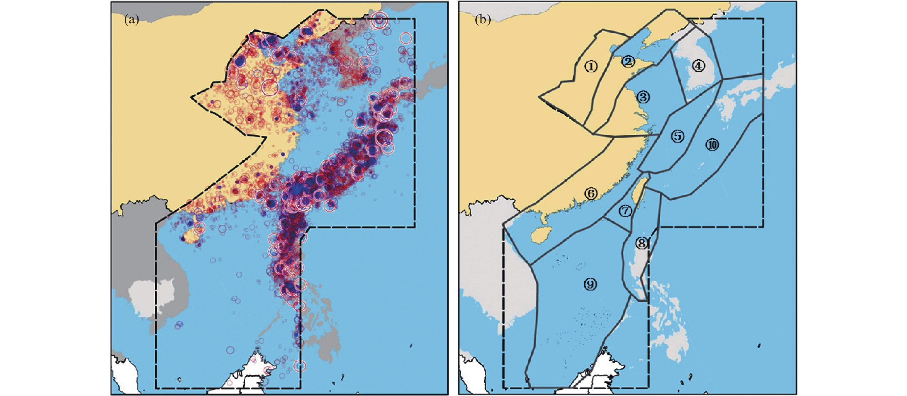
图 1 中国海域及邻区地震分布
注:(a)图中红色圆圈为主震,蓝色圆圈为余震;(b)图为近海大陆架各地震带范围,其中,①为华北平原地震带;②为郯庐地震带;③为长江下游-南黄海地震带;④为朝鲜地震带;⑤为东海地震统计区;⑥为华南沿海地震带;⑦为台湾西部地震带;⑧为台湾-马尼拉地震带;⑨为南海地震统计区;⑩为琉球海沟地震带
Figure 1. Earthquake distribution in China sea areas and adjacent areas
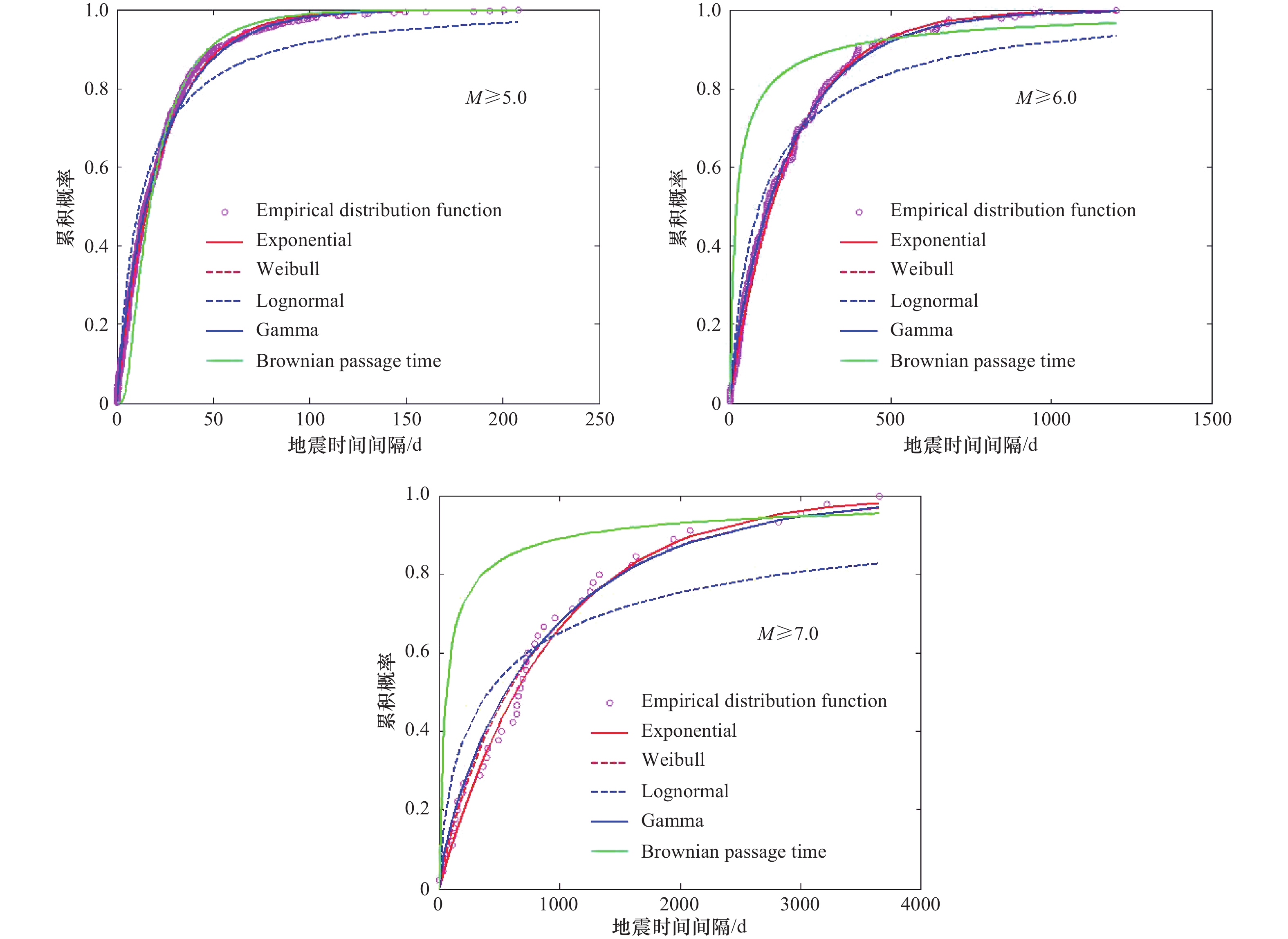
图 2 中国海域及邻区不同震级地震的时间间隔累积经验分布函数及其对应的5个模型累积分布函数
Figure 2. The cumulative empirical distribution function of the time interval of M≥5, 6, 7 earthquakes in the Sea area of China and adjacent areas and the cumulative distribution function of the corresponding five models
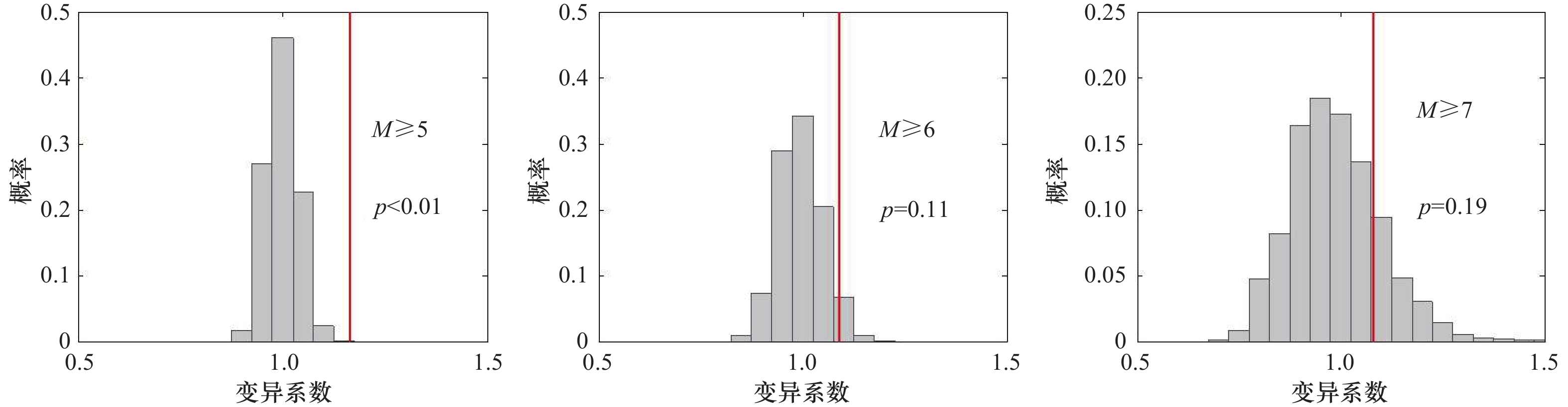
图 3 海域地震时间间隔变异系数与泊松模型变异系数对比
注:红线为实际地震记录计算的变异系数,直方图为蒙特卡洛模拟1000次泊松过程的变异系数分布
Figure 3. Comparison between the variation coefficient of sea area earthquake time interval and the variation coefficient of Poisson model

图 4 整个海域地震的扩散熵和标准差随时间变化及其标度值
Figure 4. Diffusion entropy and standard deviation of earthquakes as the function of time in the whole sea area and the scale values
表 1 中国海域及邻区模型参数及AIC、BIC和K-S检验值
Table 1. Model parameters and AIC, BIC and K-S test results for earthquakes in China Sea and adjacent areas
震级 模型 模型参数 −lnL AIC BIC K-S检值验 指数分布 μ=23.2760 ― 2770.4772 5542.9545 5547.4587 0.0366 威布尔分布 α=22.1757 β=0.9038 2764.3739 5532.7479 5541.7565 0.0384 1976年以来M≥5 对数正态分布 μ=2.4560 σ=1.5526 2882.3087 5768.6174 5777.6260 0.1067 伽马分布 α=0.8514 λ=27.3383 2764.4759 5532.9518 5541.9604 0.0391 布朗过程时间分布 μ=23.2760 α=0.0329 4548.7329 9101.4659 9110.4745 0.1667 指数分布 μ=188.8710 ― 1422.9627 2847.9253 2851.3547 0.0471 威布尔分布 α=180.4296 β=0.9047 1421.0141 2846.0283 2852.8870 0.0476 1900年以来M≥6 对数正态分布 μ=4.5348 σ=1.7015 1478.6316 2961.2631 2968.1218 0.1144 伽马分布 α=0.8355 λ=226.0487 1420.3845 2844.7689 2851.6276 0.0541 布朗过程时间分布 μ=188.8710 α=0.0874 2152.2080 4308.4161 4315.2748 0.4251 指数分布 μ=920.4309 ― 352.1179 706.2358 708.0424 0.0857 1900年以来M≥7 威布尔分布 α=869.2773 β=0.8697 351.4152 706.8304 710.4438 0.1214 对数正态分布 μ=6.0154 σ=12.3052 372.1317 748.2635 751.8768 0.2007 伽马分布 α=0.7408 λ=1242.5236 350.6158 705.2316 708.8449 0.1290 布朗过程时间分布 μ=920.4309 α=0.0344 545.7260 1095.4521 1099.0654 0.5404  下载: 导出CSV
表 2 华南沿海地震带模型参数及AIC、BIC和K-S检验值
Table 2. Model parameters and AIC, BIC and K-S test results for earthquakes in South China Coastal seismic zone
震级 分布模型 模型参数值 −lnL AIC BIC K-S检验值 1970年以来M≥4 指数分布 μ=124.1940 ― 820.8802 1643.7603 1646.7091 0.0524 威布尔分布 α=119.3586 β=0.9161 819.9501 1643.9002 1649.7977 0.0428 对数正态分布 μ=4.1325 σ=11.6783 855.7540 1715.5080 1721.4055 0.1243 伽马分布 α=0.8537 λ=145.4822 819.6564 1643.3129 1649.2104 0.0481 布朗过程时间分布 μ=124.1940 α=0.1551 1205.4927 2414.9854 2420.8829 0.8448 1900年以来M≥5 指数分布 μ=1095.4519 ― 295.9601 593.9202 595.5312 0.1106 威布尔分布 α=1070.9469 β=0.9473 295.8694 595.7388 598.9607 0.1293 对数正态分布 μ=6.3317 σ=11.5744 303.5748 611.1497 614.3715 0.2180 伽马分布 α=0.8788 λ=1246.5401 295.7488 595.4976 598.7195 0.1382 布朗过程时间分布 μ=1095.4519 α=0.20633 327.2432 658.4864 661.7083 0.5460 1900年以来M≥6 指数分布 μ=3647.1044 ― 82.8152 167.6304 167.8276 0.1553 威布尔分布 α=3876.6133 β=1.1812 82.6192 169.2384 169.6329 0.1896 对数正态分布 μ=7.8006 σ=10.9423 82.4707 168.9414 169.3359 0.1443 伽马分布 α=1.3897 λ=2624.4039 82.5429 169.0858 169.4803 0.1870 布朗过程时间分布 μ=3647.1044 α=0.5123.8113 82.5444 169.0887 169.4832 0.1601
下载: 导出CSV
表 3 台湾西部地震带模型参数及AIC、BIC和K-S检验值
Table 3. Model parameters and AIC, BIC and K-S test results for earthquakes in the western Taiwan earthquake zone
震级 分布模型 模型参数值 −lnL AIC BIC K-S检验值 1970年以来M≥4 指数分布 μ=63.9192 ― 1413.1877 2828.3755 2831.9886 0.0321 威布尔分布 α=62.5341 β=0.9513 1412.6234 2829.2469 2836.4731 0.0413 对数正态分布 μ=3.5179 σ=1.4155 1447.9090 2899.8181 2907.0443 0.0801 伽马分布 α=0.9123 λ=70.0631 1412.4117 2828.8235 2836.0498 0.0396 布朗过程时间分布 μ=63.9192 α=2.0285 1737.7414 3479.4829 3486.7091 0.5304 1900年以来M≥5 指数分布 μ=360.3387 ― 812.6713 1627.3425 1630.1132 0.0691 韦伯分布 α=349.6849 β=0.9394 812.2484 1628.4968 1634.0381 0.0627 对数正态分布 μ=5.2615 σ=1.4189 829.5743 1663.1486 1668.6900 0.1093 伽马分布 α=0.9307 λ=387.1736 812.4684 1628.9368 1634.4782 0.0650 布朗过程时间分布 μ=360.3387 α=2.3725 1047.7444 2099.4887 2105.0301 0.7232 1900年以来M≥6 指数分布 μ=1540.5848 ― 225.1778 452.3555 453.6514 0.1196 韦伯分布 α=1528.7487 β=0.9856 225.1718 454.3435 456.9352 0.1177 对数正态分布 μ=6.8444 σ=0.9483 221.6868 447.3737 449.9653 0.0680 伽马分布 α=1.1471 λ=1343.0297 225.0235 454.0470 456.6387 0.1230 布朗过程时间分布 μ=1540.5848 α=0.4539 221.4897 446.9793 449.5710 0.0680
下载: 导出CSV
表 4 台湾-马尼拉海沟地震带模型参数及AIC、BIC和K-S检验值
Table 4. Model parameters and AIC, BIC and K-S test results for earthquakes in Taiwan - Manila trench seismic zone
震级 分布模型 模型参数值 −lnL AIC BIC K-S检验值 1900年以来M≥5 指数分布 μ=198.7702 ― 1365.3964 2732.7928 2736.1727 0.1098 威布尔分布 α=172.2580 β=0.7822 1352.9227 2709.8454 2716.6052 0.0247 对数正态分布 μ=4.4145 σ=1.6354 1372.5919 2749.1837 2755.9435 0.0912 伽马分布 α=0.6900 λ=288.0880 1353.9309 2711.8617 2718.6215 0.0348 布朗过程时间分布 μ=198.7702 α=5.1720 1566.5258 3137.0516 3143.8114 0.4935 1900年以来M≥6 指数分布 μ=530.8835 ― 589.2379 1180.4759 1182.8703 0.0686 威布尔分布 α=525.5586 β=0.9762 589.2005 1182.4010 1187.1899 0.0720 对数正态分布 μ=5.6565 σ=1.3571 597.8469 1199.6937 1204.4826 0.1442 伽马分布 α=0.9408 λ=564.3035 589.1379 1182.2757 1187.0646 0.0745 布朗过程时间分布 μ=530.8835 α=1.9082 623.7724 1251.5448 1256.3337 0.3173 1900年以来M≥7 指数分布 μ=2534.7483 ― 132.5677 267.1355 267.8435 0.1465 威布尔分布 α=2598.8333 β=1.0804 132.5075 269.0151 270.4312 0.1351 对数正态分布 μ=7.2616 σ=1.4120 135.4003 274.8006 276.2167 0.1871 伽马分布 α=1.0014 λ=2531.1015 132.5677 269.1355 270.5516 0.1464 布朗过程时间分布 μ=2534.7483 α=0.8039 139.9211 283.8422 285.2583 0.3793
下载: 导出CSV
表 5 各地震带不同起始震级地震目录的扩散熵分析法和标准差分析法标度值
Table 5. DEA and SDA scale values of earthquake catalogs with different initial magnitudes in each seismic zone
地震带 M≥4 M≥5 M≥6 M≥7 δ H δ H δ H δ H 华南沿海地震带 0.56 0.58 0.37 0.46 0.38 0.46 ― ― 长江下游-南黄海地震带 0.44 0.44 0.54 0.58 0.42 0.51 ― ― 台湾西部地震带 0.47 0.47 0.65 0.74 0.56 0.64 ― ― 马尼拉海沟地震带 ― ― 0.59 0.77 0.50 0.57 0.45 0.46 琉球海沟地震带 ― ― ― ― 0.50 0.51 0.56 0.63
下载: 导出CSV
-
[1] 高孟潭, 1996. 基于泊松分布的地震烈度发生概率模型. 中国地震, 12(2): 195—201.Gao M T., 1996. Occurrence probability model of earthquake intensity based on the Poisson distribution. Earthquake Research in China, 12(2): 195—201. (in Chinese) [2] 胡聿贤, 1990. 地震危险性分析中的综合概率法. 北京: 地震出版社. [3] 潘华, 高孟潭, 谢富仁, 2013. 新版地震区划图地震活动性模型与参数确定. 震灾防御技术, 8(1): 11—23. doi: 10.3969/j.issn.1673-5722.2013.01.002Pan H., Gao M. T., Xie F. R., 2013. The earthquake activity model and seismicity parameters in the new seismic hazard map of China. Technology for Earthquake Disaster Prevention, 8(1): 11—23. (in Chinese) doi: 10.3969/j.issn.1673-5722.2013.01.002 [4] Bajaj S., Lal Sharma M., 2019. Modeling earthquake recurrence in the Himalayan seismic belt using time-dependent stochastic models: implications for future seismic hazards. Pure and Applied Geophysics, 176(12): 5261—5278. doi: 10.1007/s00024-019-02270-9 [5] Bufe C. G., Perkins D. M., 2005. Evidence for a global seismic-moment release sequence. Bulletin of the Seismological Society of America, 95(3): 833—843. doi: 10.1785/0120040110 [6] Console R., Murru M., Lombardi A. M., 2003. Refining earthquake clustering models. Journal of Geophysical Research, 108(B10): 2468. [7] Cornell C. A., 1968. Engineering seismic risk analysis. Bulletin of the Seismological Society of America, 58(5): 1583—1606. [8] Daub E. G., Ben-Naim E., Guyer R. A., et al., 2012. Are megaquakes clustered? Geophysical Research Letters, 39(6): L06308. [9] Ellsworth W. L., Llenos A. L., McGarr A. F., et al., 2015. Increasing seismicity in the U.S. midcontinent: implications for earthquake hazard. The Leading Edge, 34(6): 618—626. doi: 10.1190/tle34060618.1 [10] Gardner J. K., Knopoff L., 1974. Is the sequence of earthquakes in southern California, with aftershocks removed, Poissonian? Bulletin of the Seismological Society of America, 64(5): 1363—1367. [11] Hebden J. S., Stein S., 2009. Time-dependent seismic hazard maps for the new Madrid seismic zone and Charleston, South Carolina, Areas. Seismological Research Letters, 80(1): 12—20. doi: 10.1785/gssrl.80.1.12 [12] Jiménez, A., Tiampo, K. F., Levin, S., et al., 2006. Testing the persistence in earthquake catalogs: the Iberian Peninsula. EPL (Europhysics Letters), 73(2): 171—177. doi: 10.1209/epl/i2005-10383-8 [13] Kagan Y. Y., 1997. Statistical aspects of Parkfield earthquake sequence and Parkfield prediction experiment. Tectonophysics, 270(3—4): 207—219. [14] Kulkarni R., Wong I., Zachariasen J., et al., 2013. Statistical analyses of great earthquake recurrence along the Cascadia Subduction zone. Bulletin of the Seismological Society of America, 103(6): 3205—3221. doi: 10.1785/0120120105 [15] Mandelbrot B. B., 1982. The fractal geometry of nature. New York: W.H. Freeman and Company. [16] Matthews M. V., Ellsworth W. L., Reasenberg P. A., 2002. A Brownian model for recurrent earthquakes. Bulletin of the Seismological Society of America, 92(6): 2233—2250. doi: 10.1785/0120010267 [17] Mega M. S., Allegrini P., Grigolini P., et al., 2003. Power-law time distribution of large earthquakes. Physical Review Letters, 90(18): 188501. doi: 10.1103/PhysRevLett.90.188501 [18] Michael A. J., 2011. Random variability explains apparent global clustering of large earthquakes. Geophysical Research Letters, 38(21): L21301. [19] Nishenko S. P., Buland, R., 1987. A generic recurrence interval distribution for earthquake forecasting. Bulletin of the Seismological Society of America, 77(4): 1382—1399. [20] Ogata Y., Abe K., 1991. Some statistical features of the long-term variation of the global and regional seismic activity. International Statistical Review, 59(2):139—161. doi: 10.2307/1403440 [21] Parsons T., Geist E. L., 2012. Were global M≥8.3 earthquake time intervals random between 1900 and 2011? Bulletin of the Seismological Society of America, 102(4): 1583—1592. doi: 10.1785/0120110282 [22] Pasari S., Dikshit O., 2015. Distribution of earthquake interevent times in northeast India and adjoining regions. Pure and Applied Geophysics, 172(10): 2533—2544. doi: 10.1007/s00024-014-0776-0 [23] Pasari S., Dikshit O., 2018. Stochastic earthquake interevent time modeling from exponentiated Weibull distributions. Natural Hazards, 90(2): 823—842. doi: 10.1007/s11069-017-3074-1 [24] Petersen M. D., Moschetti M. P., Powers P. M., et al., 2014. Documentation for the 2014 update of the United States national seismic hazard maps. Reston: U.S. Geological Survey. [25] Reid H. F., 1910. The mechanics of the earthquake, the California earthquake of April 18, 1906, report of the state earthquake investigation commission, Vol. 2. Washington: Carnegie Institution of Washington. [26] Salditch L., Stein S., Neely J., et al., 2020. Earthquake supercycles and long-term fault memory. Tectonophysics, 774: 228289. doi: 10.1016/j.tecto.2019.228289 [27] Scafetta N., West B. J., 2004. Multiscaling comparative analysis of time series and a discussion on “earthquake conversations” in California. Physical Review Letters, 92(13): 138501. doi: 10.1103/PhysRevLett.92.138501 [28] Schwartz D. P., Coppersmith K. J., 1984. Fault behavior and characteristic earthquakes: examples from the Wasatch and San Andreas fault zones. Journal of Geophysical Research, 89(B7): 5681—5698. doi: 10.1029/JB089iB07p05681 [29] Shannon C., 1948. A mathematical theory of communication. Bell System Technical Journal, 27(4): 623—656. doi: 10.1002/j.1538-7305.1948.tb00917.x [30] Sharma M. L., Kumar R., 2010. Estimation and implementations of conditional probabilities of occurrence of moderate earthquakes in India. Indian Journal of Science and Technology, 3(7): 807—816. doi: 10.17485/ijst/2010/v3i7.12 [31] Shearer P. M., Stark P. B., 2012. Global risk of big earthquakes has not recently increased. Proceedings of the National Academy of Sciences of the United States of America, 109(3): 717—721. doi: 10.1073/pnas.1118525109 [32] Tripathi J. N., 2006. Probabilistic assessment of earthquake recurrence in the January 26, 2001 earthquake region of Gujrat, India. Journal of Seismology, 10(1): 119—130. doi: 10.1007/s10950-005-9004-9 [33] Tsai C. Y., Shieh C. F., 2008. A study of the time distribution of inter-cluster earthquakes in Taiwan. Physica A: Statistical Mechanics and its Applications, 387(22): 5561—5566. doi: 10.1016/j.physa.2008.05.023 [34] Utsu T., 1984. Estimation of parameters for recurrence models of earthquakes. Bulletin of the Earthquake Research Institute, University of Tokyo, 59(1): 53—66. [35] Weibull W., Sweden S., 1951. A statistical distribution function of wide applicability. Journal of Applied Mechanics, 18(3): 293—297. doi: 10.1115/1.4010337 [36] Working Group on California Earthquake Probabilities, 2013. The uniform California earthquake rupture forecast version 3 (UCERF 3)—The Time-Independent Model. (2013-11-05). http://pubs.usgs.gov/of/2013/1165/. [37] Xie Z. J., Li S. Y., Lyu Y. J., et al. 2021. Empirical relations for conversion of surface- and body-wave magnitudes to moment magnitudes in China’s seas and adjacent areas. Journal of Seismology, 25(1): 213–233. doi: 10.1007/s10950-020-09947-y [38] Zhou Y., Chechkin A., Sokolov I. M., et al., 2016. A model of return intervals between earthquake events. EPL (Europhysics Letters), 114(6): 60003. doi: 10.1209/0295-5075/114/60003 [39] Zinn-Justin J., 2002. Quantum field theory and critical phenomena. 4th ed. Oxford: Oxford University Press. -

 点击查看大图
计量
- 文章访问数: 574
- HTML全文浏览量: 74
- PDF下载量: 41
- 被引次数: 0
