
A New Explicit Time Integration Algorithm for Nonlinear Seismic Response Analysis of Site
-
摘要: 针对线弹性结构动力学方程,作者已提出一种具有良好稳定性的二阶精度单步显式时间积分算法。本文将该方法推广到求解材料非线性结构动力学方程中,采用带误差控制的修正欧拉算法计算单元应力,提高显式时间积分算法的精度。将求解非线性问题的显式算法应用于地震波垂直入射时非线性地震反应分析中,使用黏性边界模拟场地土层底部半空间基岩的辐射阻尼,并考虑地震动输入。与中心差分法计算结果进行对比,以表明新显式算法的有效性。Abstract: For the linear-elastic structure dynamics equation, the author has proposed a second-order precision single-step explicit time integration algorithm with good stability. In this paper, the method is extended to solve the nonlinear structural dynamics equations, and the modified Euler algorithm with error control is used to calculate the element stress and improve the accuracy of the explicit time integration algorithm. The explicit algorithm for solving nonlinear problems is applied to nonlinear site seismic response analysis. The viscous boundary is used to simulate the radiation damping of the bedrock underlying the soil layer, and the ground motion input is considered. The comparison with the calculation results of the central difference method shows the effectiveness of the new explicit algorithm.
-

图 2 大开车站沿线土层纵断面构造
Figure 2. Site condition of the Daikai subway station in vertical direction
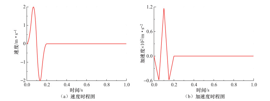
图 3 狄拉克脉冲速度和加速度时程图
Figure 3. Velocity and acceleration time history of the Dirac pulse
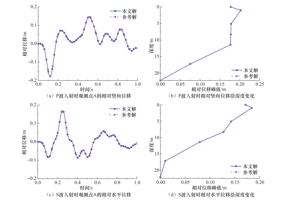
图 4 狄拉克脉冲入射时场地反应分析结果
Figure 4. Results of site analysis under the incident of Dirac pulse
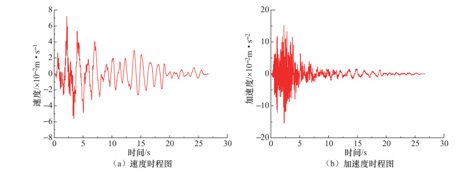
图 5 实测地震动速度和加速度时程图
Figure 5. Velocity and acceleration time history of the seismic motion
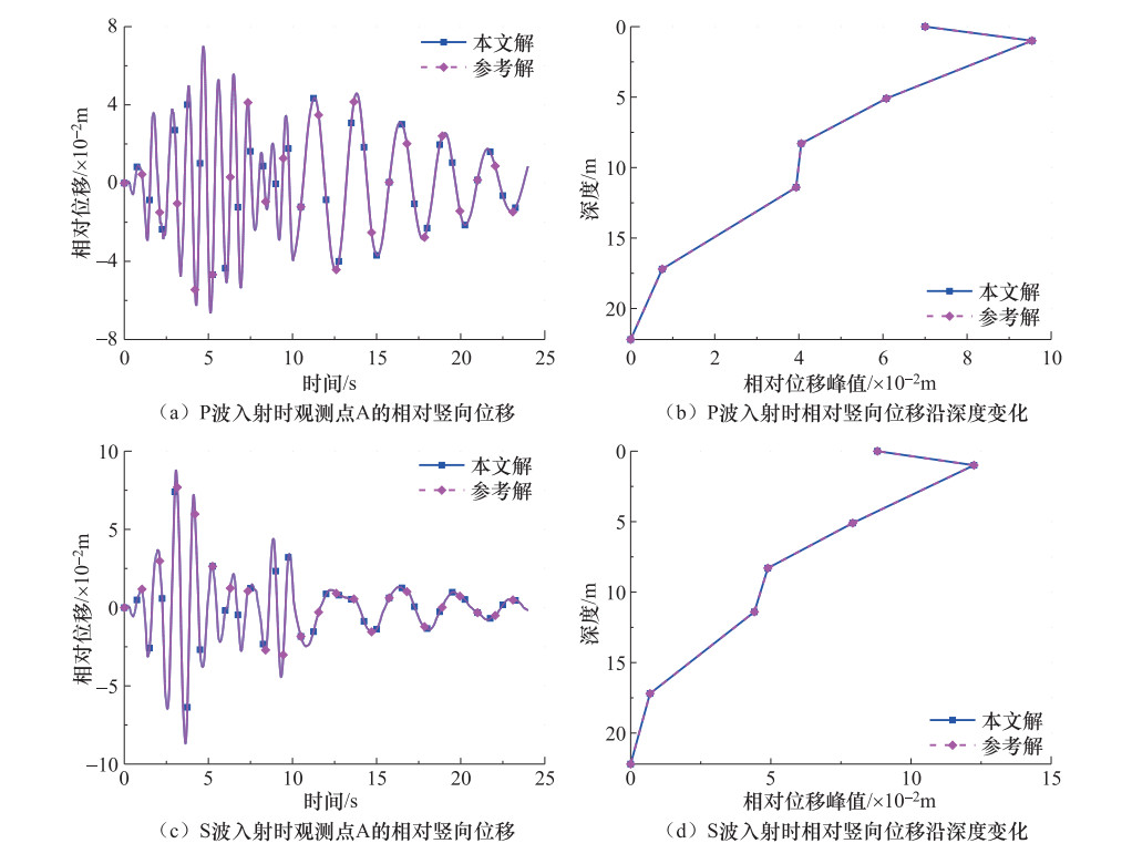
图 6 实测地震动入射时场地反应分析结果
Figure 6. Results of site reaction analysis under the incident of the seismic motion
表 1 土层参数
Table 1. Parameters of soils
土质 深度/
m$\rho $/
(g/cm3)cs /
(m/s)v
-EN
-Rf
-c/
(MPa)θ/(°) D
-F
-人工填土 0—1.0 1.9 140 0.33 0.33 0.758 0.084 26.9 1.06 0.021 全新世砂土 1.0—5.1 1.9 140 0.32 0.33 0.758 0.084 26.9 1.06 0.021 全新世砂土 5.1—8.3 1.9 170 0.32 0.36 0.768 0.120 31.0 1.11 0.015 更新世粘土 8.3—11.4 1.9 190 0.40 0.44 0.822 0.188 28.4 1.01 0.012 更新世粘土 11.4—17.2 1.9 240 0.30 0.44 0.822 0.188 28.4 1.01 0.012 更新世砂土 17.2—22.2 2.0 330 0.26 0.51 0.840 0.300 30.0 1.02 0.011 基岩 >22.2 2.0 330 0.26 - - - - - -  下载: 导出CSV
-
杜修力, 李洋, 许成顺等, 2016.1995年日本阪神地震大开地铁车站震害原因及成灾机理分析研究进展.岩土工程学报, 40(2):223-236. http://d.old.wanfangdata.com.cn/Periodical/ytgcxb201802002 栾茂田, 林皋, 1992.场地地震反应一维非线性计算模型.工程力学, 9(1):94-103. http://www.cnki.com.cn/Article/CJFDTotal-GCLX199201015.htm 王笃国, 赵成刚, 2016.地震波斜入射时二维成层介质自由场求解的等效线性化方法.岩土工程学报, 38(3):554-561. http://d.old.wanfangdata.com.cn/Periodical/ytgcxb201603020 王进廷, 杜修力, 2002.有阻尼体系动力分析的一种显式差分法.工程力学, 19(3):109-112. http://d.old.wanfangdata.com.cn/Periodical/gclx200203022 尹候权, 2015.地震波斜入射时成层半空间场地反应分析方法及其应用.北京: 北京工业大学. Ahadi A., Krenk S., 2003. Implicit integration of plasticity models for granular materials. Computer Methods in Applied Mechanics and Engineering, 192(31-32):3471-3488. http://www.wanfangdata.com.cn/details/detail.do?_type=perio&id=dd253a3e8dddeed056e6c5a8b1aa1498 Arslan H., Siyahi B., 2006. A comparative study on linear and nonlinear site response analysis. Environmental Geology, 50(8):1193-1200. doi: 10.1007/s00254-006-0291-4 Bardet J. P., Ichii K., Lin C. H., 2000. EERA-A computer program for equivalent-linear earthquake site response analyses of layered soil deposits. Belytschko T., Liu W. K., Moran B., et al., 2014. Nonlinear finite elements for continua and structures. 2nd updated and extended ed. John Wiley & Sons Inc. Chopra A. K., 2009. Dynamics of structures: Theory and applications to earthquake engineering (3rd edn). Tsinghua University Press: Beijing. Chung J., Lee J. M., 1994. A new family of explicit time integration methods for linear and non-linear structural dynamics. International Journal for Numerical Methods in Engineering, 37(23):3961-3976. doi: 10.1002/nme.1620372303 Crisfield M. A., 1991. Nonlinear finite element analysis of solids and structures. Journal of Engineering Mechanics, 17(6):1504-1505. http://d.old.wanfangdata.com.cn/OAPaper/oai_arXiv.org_1110.5321 Duncan J. M., Chang C. Y., 1970. Nonlinear analysis of stress and strain in soils. Journal of the Soil Mechanics and Foundations Division ASCE, 96(5):1629-1653. http://ci.nii.ac.jp/naid/10007805651 Hashash Y. M. A., Phillips C., Groholski D. R., 2010. Recent advances in non-linear site response analysis. Fifth International Conference on Recent Advances in Geotechnical Earthquake Engingeering and Soil Dynamics and Symposium in Honor of Professor I.M. Idriss. San Diego, California. Hosseini S. M. M. M., Pajouh M. A., 2012. Comparative study on the equivalent linear and the fully nonlinear site response analysis approaches. Arabian Journal of Geosciences, 5(4):587-597. http://www.wanfangdata.com.cn/details/detail.do?_type=perio&id=8661fab143f2e354f593dd1ff81acd3c Huang H. C., Shieh C. S., Chiu H. C., 2001. Linear and nonlinear behaviors of soft soil layers using Lotung downhole array in Taiwan. Terrestrial, Atmospheric and Oceanic Sciences, 12(3):503-524. http://www.wanfangdata.com.cn/details/detail.do?_type=perio&id=CC027479014 Idriss I. M., Sun J. I., 1992. User's Manual for SHAKE91: A computer program for conducting equivalent linear seismic response analysis of horizontally layered soil deposits. Center for Geotechnical Modeling, Department of Civil and Environmental Engineering, University of California. Joyner W. B., Chen A. T. F., 1975. Calculation of nonlinear ground response in earthquakes. Bulletin of the Seismological Society of America, 65(5):1315-1336. http://www.wanfangdata.com.cn/details/detail.do?_type=perio&id=Doaj000003603734 Schnabel P. B., Lysmer J., Seed H. B., 1972. SHAKE a computer program for earthquake response analysisi of horizontally layered sites. Report No. UBC/EERC72-12. Berkeley, USA: Earthquake Research Center, University of California. Sloan S. W., Abbo A. J., Sheng D., 2001. Refined explicit integration of elastoplastic models with automatic error control. Engineering Computations, 18(1-2):121-194. http://www.wanfangdata.com.cn/details/detail.do?_type=perio&id=76c28dcc34c077dea2b16ae6d6674092 Sloan S. W., Booker J. R., 1992. Integration of tresca and mohr-coulomb constitutive relations in plane strain elastoplasticity. International Journal for Numerical Methods in Engineering, 33(1):163-196. doi: 10.1002/nme.1620330112 Zhao M., Li H., Cao S. et al. 2019. An explicit time integration algorithm for linear and non-linear finite element analyses of dynamic and wave problems. Engineering Computations, 36(1):161-177. http://www.wanfangdata.com.cn/details/detail.do?_type=perio&id=497e43137d940ce8f0a85b06178f0517 -

 点击查看大图
计量
- 文章访问数: 134
- HTML全文浏览量: 85
- PDF下载量: 3
- 被引次数: 0
